Linked List:
Linked list or one way
list is a linear collection of data elements, called nodes. Where linear order
is given by means of pointers. Each node is divided into two parts:
· The first part contains
the information of the element.
· The second part called
the link field or the next pointer field contains the address of the next
element in the list.
Figure shows a
schematic diagram of linked list with 3 nodes
Each node is pictured with 2 parts. The left part
contains the information of the node, which may contain an entire record of
data items. The right part represents the next pointer field of the node. The pointer of the last node contains a
special value, called null pointer, which is having an invalid address.
In actual practice, 0 or a negative number used for
the null pointer. The null pointer signals the end of the list. The linked list also contains a list pointer
variable- START or Head- which contains the address of the first node in the
list. There is an arrow drawn from the
start with the first node.
A special case is the list has no nodes, such list is called null list or empty list and is denoted by the null pointer in variable START or Head.
Representation of Linked List in memory:
Let list be a linked list.
The list will be maintained in memory, we require two linear arrays to
store information and link the pointer field of the node in the list. List also require a pointer variable start
which contains the location of the beginning of the list and next pointer
sentinel denoted by NULL-which indicates the end of the list
Traversing a Linked List:
Let List be a linked list in memory stored in a linear array INFO and
LINK with start pointing to the first element and NULL indicates the end of the
list. Suppose we want to traverse lists in order to process each node exactly
once.
Traversing
algorithm uses a pointer variable PTR which points to the node that is
currently being processed. Accordingly, the LINK[PTR] points to the next node
to be processed. Thus the assignment:
PTR: =LINK[ PTR]
Move the pointer to the next node in the list
Algorithm:
(Traversing) Let List be a linked list in memory. This algorithm
traverses a list. Applying an operation to process each element of the list.
Variable PTR point to the node current being processed
- Set PTR:=START [initializes pointer PTR]
- Repeat steps 3 and 4 while PTR
!= NULL
- Apply process to INFO[PTR]
- Set PTR:=LINK[PTR] [ PTR now
points to next node]
[End of Step 2 loop]
- Exit
Searching a Linked List:
List is Sorted: Suppose the data in the list are
sorted. Then one searches for an item in the list by Traversing into a list
using the pointer variable PTR and comparing the item with the content of INFO[PTR]
of each node, one by one, of the list.
PTR:=LINK[PTR]
We require two tests. First we have to check to see whether
we have reached the end of the list that is first we check to see whether:
PTR =NULL
If not, then we check
to see whether:
INFO[PTR]=ITEM
Algorithm: Searching (INFO, LINK, START, ITEM,
LOC)
List is a sorted list in memory. This algorithm finds the
location LOC of the node where the item first appears in the list or sets
LOC=NULL.
1. Set
PTR:=START [initializes pointer PTR]
2. Repeat steps 3 while PTR != NULL
3. If ITEM < INFO[PTR], then:
Set PTR:=LINK[PTR] [PTR now points to next node]
Else if ITEM=INFO[PTR], then:
Set LOC:=PTR, and exit
[Search is Successful]
Else
Set LOC:=NULL. And exit
[ITEM now exceeds INFO[PTR]]
[End of if Structure]
[End of Step 2 Loop]
4. Set LOC:=NULL
5. Exit
Memory Allocation:
The maintenance of the linked list in memory assumes the
possibility of inserting new node into the list and hence required some
mechanism which provides unused memory space for the new node
Some mechanism is required hereby the memory space of the
deleted node becomes available for future use
Together with the
linked list in memory, special this is maintained which consists of the unused
memory cell, which has its own pointer, is called the list of
available space or storage list or free pool
Garbage Collection:
The operating system of the
computer periodically collects all the deleted space into a free storage list.
Any technique which does this collection is called garbage collection.
Garbage Collection usually takes
place in two steps. First the computer runs through all the list, tagging those
cells which are currently in use, and then the computer runs through the memory
and collects all the untagged space onto the free storage list. The garbage
collection method takes place when there is only some minimum amount of space
or no space left in a free storage list, or when the CPU is idle and has time
to do the collection. Generally speaking garbage collection is invisible to the
programmer.
Overflow and Underflow
Sometimes new data is to be inserted into a
data structure but there is no available space that is a free storage list is
empty. This situation is usually called Overflow. The programmer may handle the overflow by
printing the message overflow. In such
cases the programmer modified the program by adding space to the underlying
array. Observe that overflow-will occur with our linked list when AVAIL=NULL
and at the time of insertion.
The term Underflow
refers to the situation where we want to delete the data from a data structure
that is empty. A programmer may handle
underflow by printing message underflow.
Observe that underflow will occur with our linked list in START= NULL
and at the time of deletion.
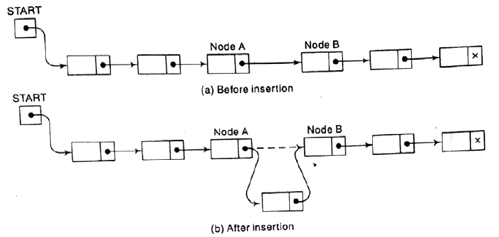
Insertion into a linked list:
Let the list be linked with successive
nodes and A and B shown in figure. Suppose in node and is to be inserted into a
linked list between node A and node B.
Suppose our linked list is
maintained in memory in the form
LIST(INFO, LINK, START,
AVAIL)
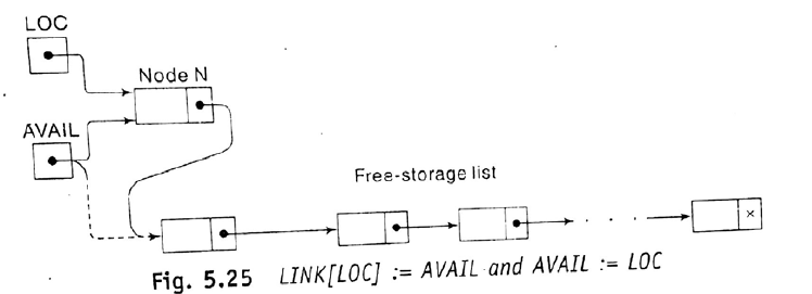
- The
next pointer field of node N now points to new node N, to which AVAIL
previously pointed.
- AVAIL
now points to the second node in the free pool,, to which node N
previously pointed
- The next pointer field of node N now
points to node B, to which node A previously pointed.
Insertion algorithms:
- Checking
to see if the space is available in the AVAIL list. if not, that is, if AVAIL=NULL then the
algorithm will print the message
overflow.
- Removing
the first node from the AVAIL list. Using the variable NEW to keep track
of the location of the new node, this type can be implemented by the pair
of assignment
NEW:=AVAIL,
AVAIL:=LINK[AVAIL]
3. Copying new information into
new node:
INFO[NEW]:=ITEM
Inserting at the Beginning of the
list:
Algorithm: INSBEG(INFO,LINK START,
AVAIL, ITEM)
This algorithm inserts ITEM as the
first node in the list.
- [OVERFLOW?]
If AVAIL=NULL, then: Write: OVERFLOW, and Exit.
- [Remove
first node from AVAIL list]
Set
NEW:=AVAIL and AVAIL:=LINK[AVAIL]
- Set
INFO[NEW]:=ITEM [Copies new data into new node]
- Set
LINK[NEW]:=START [New node now points to original first]
- Set
START:=NEW. [Changes START so it points to the new node]
- Exit.

Inserting after a given node:
Suppose we are given the value of
LOC where LOC is a location of a node in a linked list or LOC = NULL. This algorithm inserts ITEM into a list so
that item follows node A or when LOC = NULL so that item is the first node.
Let N denote the new node. if LOC=NULL, then N is inserted as the first
node in the list.
Let node N point to node B:
LINK[NEW]:=LINK[LOC]
And we let node A points to new
node N by the assignment
LINK[LOC]:=NEW
Algorithm: INSLOC (INFO, LINK, START, AVAIL, LOC, ITEM)
- [OVERFLOW?]
If AVAIL=NULL, then: Write: OVERFLOW, and Exit.
- [Remove
first node from AVAIL list]
Set
NEW:=AVAIL and AVAIL:=LINK[AVAIL]
- Set
INFO[NEW]:=ITEM [Copies new data into new node]
- If
LOC= NULL , then: [insert as a first node]
Set LINK[NEW}:= START and START:= NEW
Else:
[insert after node with location LOC]
Set
LINK[NEW]:=LINK[LOC] and LINK[LOC]:= NEW
[End
of If structure]
- Exit.